Multiposition Synthetic Aperture Radar (MPSAR) 

              Alexander V Ksendzuk 

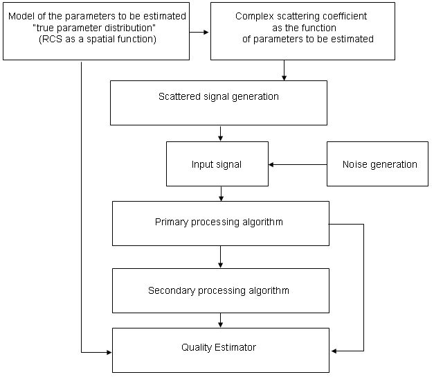
10. Multiposition SAR. Modeling principles.

Why the model not real data? There are two main reasons:

1.      Real SAR/radar experiment is much more expensive than modelling.

2.      One “quite good” model may be changed to analyse in other conditions or to analyse other systems.

3.      If we process real data with different primary (estimation information from the input signal) and secondary (processing of the radar images) we just can say “it is different” because we don’t know “real values”. Therefore modelling allows to estimate errors of different algorithms because we know “true”.

 In this section modelling principles are discussed.

           10.1. General Modeling Algorithm.

Estimation any other parameters even non-stationary in time, but for clarity we consider RCS estimation of the stationary scene).

Modelling algorithm is shown in Fig. 10.1.

RCS as the spatial function may be represented by any random or deterministic function but usually real radar images are used.

Complex scattering coefficient is a spatial function value of which presents in signal model (see equation 2.1 in Signal Model section). Behaviour of the complex scattering coefficient as the function of the surface parameters can be represented by functionally-determined of stochastic models (see 2.2, 2.3 in Signal Model section).

Scattered from the surface  signal must be generated for given spatial configuration with usage of the complex scattering coefficient (see equations  2.2, 2.1 in Signal Model section).

Input signal is an addition of the scattered signal and noise which may be natural or artificial. Natural noise usually approximated by Gaussian model, artificial – by other stochastic models (random pulses, Rayleigh distribution etc.).

Signal Groups in Multiposition SAR

Then any primary processing algorithms  applies to the input signal. Result of this processing is estimated value which can be compared with “true distribution”.

Different secondary processing algorithms (smoothing of the radar image) can be compared by estimation errors which are calculated in Quality Estimator. 

Figure 10.1. Synthetic Aperture Radar Modeling algorithm

10.2. Surface model.

             Surface model was described in section Signal Model.  General idea is generation of the complex scattering coefficient due to selected surface model (functionally-determined or stochastic).

Here we describe simplified stochastic surface model.

As was mentioned above accurate relations between received signal and surface parameters can be derived by means of electromagnetic equations for the selected surface model (functional-determined models). However, in common case solution of these equation  is very difficult, especially for the real, complicated surfaces.

Despite of functional-determined surface models, stochastic surface model are characterised by random fluctuations of the scattered electromagnetic field.

It is difficult to give adequate definition of these processes, so usually real scene is represented by some simplified models. One of these models is assuming surface as a set of elementary (point) scatterers with random dispositions and own reflection’s probability distribution.

Complex scattering coefficient with this model is a sum of the complex independent delta-correlated non-stationary processes, statistical characteristic of which is the radar cross section . Statistical relation between   and  is given by

                                                (10.1)

where -statistical averaging; - space delta-function.

One of the  models is its representation by the Gaussian delta-correlated non-stationary space process

,                                                       (10.2)

                                                        (10.3)

where              - are the real and imaginary parts;  - space functions, which must satisfy (1); ,  - independent Gaussian delta-correlated space processes with zero mean.

 Amplitude and phase distributions of the  are given by:

. (10.4)

This model is quite adequate if inside resolution interval there are many elementary scatterers for given wavelength and SAR parameters. In common case it is necessary to use more complicated model when process  will be non-Gaussian or Gaussian with correlation function which depends on surface behaviour (for example delta-correlated for the grass or forest, with small correlation interval for “sharp” surfaces such as tillage etc.).

Distribution of the   (model of the primary processing output) will be Gaussian, covariance functions of the real, imaginary and real-imaginary parts will be:

,

,

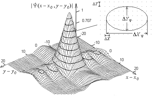
As we can see from the equations above, common-used distribution for the SAR image interpretation (Raleigh, Gaussian etc.) may be achieved from the last equation with different parameters. It is necessary to emphasize that different distributions come with different RCS behaviour as well as with different SAR space ambiguity function.

Sampling in time domain must satisfy sampling theorem, sampling rate must be chosen due to resolution of the SAR to be modelled (I recommend to choose at least 10 per 10 points in resolution cell), Figure 10.2.

Figure 10.2. Resolution and sampling rate in space domain.

10.3.   Input signal modelling 

IInput signal in the antenna may be written for the continuous transmitted signal as follows:

,    (10.5)

where              - denotes antenna pattern;  - complex envelope of the signal;  -  time delay; - carrier frequency;          - additive noise, later Gaussian with zero mean and correlation function .

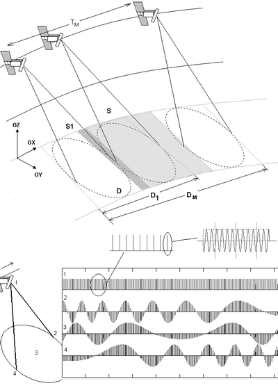
Sampling in time domain must satisfy sampling theorem (time sampling depends on signal model – complex envelope or signal with carrier frequency usage in equation 10.5). Total length of the signal in time domain depends on image size, Figure 10.3.

Figure 10.3. Signal length and sampling rate in time domain.

With the stochastic surface models input signal in the antenna  may be considered as a non-stationary Gaussian process. It is well-known that for description of such processes it is enough to find first two statistical moments (covariance function and mean). These characteristics were derived as follows:

,                                                                                                           (10.6)

,            (10.7)

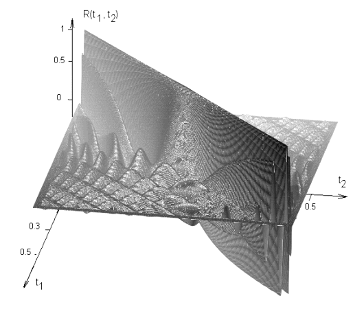
As we can see from equation (6) covariance function depends on scene parameters. An example of the correlation function (6) is shown in Figure 10.4.

Figure  10.4. Correlation function .

10.4.     Processing algorithms.

Modelling of the primary processing algorithms is processing of the discrete-time signal. Result of the processing is non-smoothed parameter estimation (spatial function) or in our case – RCS estimation.

Secondary processing algorithms is a adaptive/non-adaptive image smoothing methods, which was described in detail in lot of papers.

10.5.     Quality estimation of the processing algorithms

 Parameter estimation errors (or in considered case - image (radar cross-section) estimation errors)  are quality identifiers which allow to compare different SAR systems and/or different processing algorithms.

It is suggested to derive these errors into dynamic, fluctuation and noise errors.

Dynamic error is a distortion appeared due to smoothing with a space ambiguity function (primary processing) and smoothing windows (secondary processing).

For analytic determination of this error input process  with infinite ensemble (infinite set of the SAR channels or looks) are supposed.

Fluctuation error (in other words speckle noise or speckle) is a distortion appeared due to limited ensemble set (one realisation of the stochastic input process). For analytic determination of this error input process (2), (3) with one realisation (one-channel, one-look SAR) without additive noise and with  must be chosen.

Noise error  is a distortion appeared due to additive noise presence at the input of the system.

Total error is the distance between true and estimated values of the RCS (image) for the given radar cross-section distribution (given source image), given surface model and additive noise realisation.

A common quality criterion is a weighted sum of the dynamic, fluctuation and noise errors. This common quality criteria  can   be written as

,

where  are the  coefficients which describe appropriate noise levels.

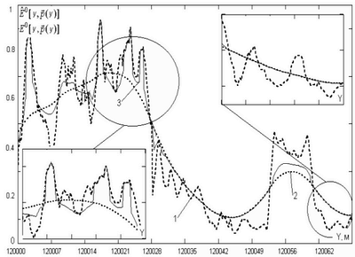
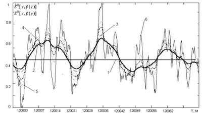
It is obvious that all of these errors depend on realisation of the radar cross-section, complex scattering coefficient and additive noise. To estimate quality of the algorithm we have to made an ensemble average of the errors. This averaging must be made for different source images (source RCS distribution), different realisation of the complex scattering coefficient as the spatial stochastic process, different additive noise realisation.

As an example, behaviour of the image formation errors for different primary processing algorithms  are shown in  Figures 10.5-10.6.

Figure 10.5.  Dynamic errors of the RCS (1) estimation for different primary processing algorithms 2 and 3.

 Figure 10.6.  Fluctuation errors of the RCS (1) estimation for different primary processing algorithms 2 and 3.

Conclusion

With proposed scattered signal model it is possible to generate SAR input signal for the real complicated surface. Input signal can be considered as a non-stationary time process connected with non-stationary space process (complex scattering coefficient) through SAR imaging parameters (antenna pattern, transmitted signal, SAR movement parameters etc). Image formation error was derived into dynamic, fluctuation and noise errors. This differentiation takes into account different basis of the errors. Dynamic caused by smoothing of the estimated parameters, fluctuation caused by finite ensemble of the non-stationary input process, noise caused by presence of the additive noise in SAR input. Proposed quality criteria allow to choose appropriate primary and/or secondary processing algorithms which provide sufficient quality of the radar image. Represented stochastic surface model and optimal processing algorithm which considers non-stationary random behaviour promises to give an advantage in SAR processing only due to algorithms enhancement. SAF of the considered algorithm narrower than SAF for the matching filtering estimator. Spatial compression of the SAF proportional to input signal SNR, the more SNR the narrower SAF.

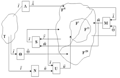
Addition. General model of the multiposition Remote sensing System.

This paper represents description and analysis method of the multiposition/ multichannel synthetic aperture radars in terms of the stochastic vector fields and operational analysis. Due to this method electrodynamic model of the surface, scattered and received signal models are considered as an operators in the function space. This allows to generalise existing methods of the description and analysis of multiposition systems.

Remote sensing in terms of the stochastic vector fields.

We denote monitoring region   as a linear space , , each element of which – vector  – is a space-time coordinates. For example, vector  in Cartesian coordinates basis will be vector , where first triplet denotes space coordinates, and the last element denotes time

Lets denote space   as a space of the linear vectors, each of coordinates is a complex continuous function quadratically integrable. Lets separate some subspaces in :  and  - subspaces of the complex and real functions,  - subspace of the vector-real functions.

We denote electrohysical parameters  of the surface as an operator  acting from  in  .

Operator  may be deterministic and stochastic as well. Vector length is restricted by the number of the electrophysical parameters, used for the description of the scattering and reflecting of the electromagnetic waves for the given surface. Most common parameters are complex permittivity, humidity, altitude etc. Dependence  allows to separate static , and dynamic  surface models.

We define operator : , acting from  in , which forms vector of the observation parameters (attitude of the receiver and transmitter, velocity vectors, frequency etc).  Model of the surface is the operator : , where  are the  vectors of the input parameters.

Vector  (output of the operator) we’ll call vector of the registered physical quantities (complex scattering coefficient and radar cross-section for the different carrier frequencies and polarizations, radio brightness and others). This vector  determines relations between registered physical quantities and electrophysical parameters.

Operator  may be deterministic (deterministic surface models) as well as stochastic (in this case we mean stochastic surface models). In the last case to each fixed value of the input parameters  correspond stochastic vector field  (some components or some coordinates of which may be deterministic).

Usually the higher number of the vectors  components the higher validity of the surface model . Physically this fact means enumeration in the surface model each possible factors of which affects on the scattered/reflected electromagnetic field.

In case of the multisatellite/multiposition radar it is useful to take into account elevation angle, carrier frequencies, polarization characteristics etc.

But during analysis and calculations it is necessary to use simplified surface models. We determine minimal sufficient surface model   for the given configuration of the multipositon radiolocation system.

To satisfy minimal  sufficient surface model  we have to eliminate from the vector  all components which are not registered, then we have to eliminate all linear dependent vectors using the rule: if  , where  is the arbitrary coefficient, element  of the  may be eleiminated without changing reliability of the model.

After series of this transformations we will achieve vector   - minimal sufficient vector of the registered physical quantities. For the  we have to denote minimal vectors of the input parameters  by elimination all components which do not effect on the  . In the final stage we should modify operator : . This model will be the minimal sufficient surface model for the given configuration of the multipositon/multichannel radiolocation system.

Signal model in the remote sensing system we will call operator  which defines relations between registered physical quantities and signal parameters  with electrophysical surface parameters .

Model of the input signal in the multisatellite radar is the stochastic vector field , which distorts useful signal. The most common model of this field is additive noise.  Usually we consider this noise to be Gaussian with zero mean and constant variance. In this case input process may be denoted as the stochastic vector field, mean of which is the useful signal, and variance depends on surface model. Generally, the noise model may be described as an operator , acting from  into . General parameters of this operator are statistical moments or the appropriate specral density coefficients  (multiscale Fourier transform of the multivariative probability density function).

Operator  determines probability functional of the input process and may be used as the basis for the optimal - estimation.

Now we can separate different tasks in the remote sensing system in the proposed terms:

З        estimation of the physical quantities (vector field  and  operator  are  given,  we have to estimate coordinates of the );

З        estimation of the registered physical quantities (vector field  and  operator  are  given,  we have to estimate coordinates  when surface model  and parameters of the observation  are known);

З        system calibration (vector field , operator , surface model  and coordinates  are known, we have to estimate , ).

Estimation mean of the stochastic vector field. Consider stochastic vector field , the task of the estimation is to find  . If we consider  to be measureable with continuous variance and   measureable and continuous for each ,  field  will be measureable on collection . In this case exists continuous bounded isotropic spectral density  and when , where - distance, - variance. From the last equation it is easy to determine boundary accuracy of the measurements in multiposition radar when received stochastic field considered to be addition of the signal and noise fields. It will be a weighted addition of the different processes in the input of the antenna, de-correlated due to space-time second-order statistic.

top